Mixture of Experts and Scaling Laws
In short: A Mixture of Experts (MoE) model has many specialist feed-forward blocks but runs only a few per token, and scaling laws tell us how much model size, data and compute we need for a given quality.
On this page
Level: Advanced · Reading time: 11 min · Phase: 3 · LLM Concepts
Before you start: Inside a Transformer Block. A mixture of experts replaces the feed-forward network described there.
Explain it like I'm new
Imagine a hospital. A dense model is a single doctor who handles every patient and must know everything. An MoE model is a hospital with 8 specialists and a receptionist (the router). Each patient (token) is sent to the 2 most suitable specialists, and their opinions are blended. The hospital employs 8 doctors (big knowledge capacity) but each patient only costs 2 doctors' time (cheap per patient).
The second half of this page answers a different question: if I have a fixed budget, should I build a bigger model or train a smaller one longer? Researchers found that quality improves along smooth, predictable curves, called scaling laws. That predictability is why labs can plan multi-million-dollar training runs.
Watch it
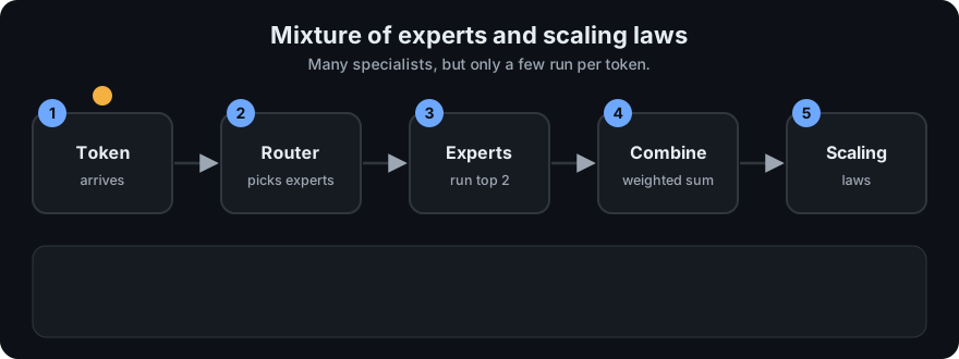
It plays on a loop. Read the caption in the box, one step at a time. Want to go at your own pace? Step through it with Previous and Next.
How it works
1. Replace the FFN with experts plus a router
In a transformer block, attention is followed by a feed-forward network (FFN). MoE (Shazeer et al., 2017; in transformers, Switch Transformer) swaps that single FFN for E expert FFNs plus a small router. Attention layers stay as they are.
flowchart LR
  T[token vector] --> R[router: one score per expert]
  R -->|softmax, top-2, renormalize| W[weights]
  T --> E1[expert 1]
  T --> E5[expert 5]
  E1 --> S[weighted sum]
  E5 --> S
  W --> S
  S --> O[layer output]
2. The router, step by step
- Score: the router gives each expert a number (a dot product between the token and the router's weights).
- Softmax: turn scores into probabilities.
- Top-k: keep the
kbest experts (commonly 1 or 2); the others do no work for this token. - Renormalize: divide the kept probabilities by their sum, so they add up to 1.
- Output = the weighted sum of the chosen experts' outputs.
Tiny worked example: probabilities [0.5, 0.3, 0.15, 0.05], top-2 keeps 0.5 and 0.3; their sum is 0.8, so the final weights are 0.625 and 0.375.
3. Total versus active parameters
All experts must exist, but a token only uses k of them. With the demo's sizes (d_model 4096, d_ff 14336, an FFN with two weight matrices, 8 experts, top-2) the module computes, for one MoE FFN layer:
| Parameters | |
|---|---|
Per expert FFN (2 × 4096 × 14336) | 117,440,512 |
Router (4096 × 8) | 32,768 |
| Total (8 experts + router) | 939,556,864 |
| Active per token (2 experts + router) | 234,913,792 |
| Active / total | 0.25 |
So the layer holds about 4x the knowledge capacity of one expert while costing roughly the compute of two. These are arithmetic on illustrative sizes, not a particular released model.
4. The load-balancing problem
Routers can be lazy: a few popular experts get most tokens, the others never learn. Then you pay for memory you do not use, and in a distributed setup the busy expert becomes a bottleneck. The demo's fixed toy router shows it on six tokens:
the -> expert 5 (w=0.52), expert 0 (w=0.48)
cat -> expert 0 (w=0.53), expert 5 (w=0.47)
sat -> expert 4 (w=0.76), expert 0 (w=0.24)
 ...
load per expert: [0.5, 0.0, 0.0, 0.0, 0.25, 0.25, 0.0, 0.0]   imbalance: 4.0
Imbalance is max load × number of experts. Perfect balance is 1.0; everything on a single expert would be 8.0. Here expert 0 handles half of all assignments and four experts get nothing, giving 4.0.
The usual cure is an auxiliary balance loss added during training. In the Switch Transformer form it is E × Σ f_e × P_e, where f_e is the fraction of tokens sent to expert e and P_e is its average router probability. It equals 1.0 when both are uniform and rises when routing collapses, so minimizing it nudges the router to spread tokens out. Many systems also cap each expert's capacity per batch.
5. Trade-offs
| Dense model | MoE model | |
|---|---|---|
| Compute per token | All parameters | Only the active ones |
| Memory for weights | Equals total | Equals total (all experts loaded) |
| Training | Simpler | Needs balancing tricks, can be less stable |
| Serving | Simple | Needs routing and often multi-GPU communication |
Key point: MoE saves compute, not memory. You still must hold every expert's weights (see quantization to shrink them).
6. Scaling laws
Kaplan et al. (2020) found that test loss falls as a power law with model parameters N, data D and compute C: roughly L = a × N^(-α). On ordinary axes this is a curve that flattens. On log-log axes (take the log of both sides) it is a straight line: log L = log a − α × log N, and the slope is −α. Fitting a line to a few small runs lets you extrapolate to a larger one.
The demo generates synthetic points from 10 × N^(-0.076) for N from 10^6 to 10^9 (made-up numbers, not real measurements; the exponent 0.076 is just an illustration) and recovers a = 10.000, α = 0.0760 using least squares on the logs.
7. The Chinchilla idea and 6·N·D
Training compute is approximately:
FLOPs ≈ 6 × N (parameters) × D (training tokens)Chinchilla (Hoffmann et al., 2022) argued that for a fixed compute budget, model size and training tokens should grow together; many earlier models were too big and under-trained. A commonly quoted rule of thumb from that paper is about 20 training tokens per parameter. The table below is arithmetic from the formula, not measured results:
| Parameters N | Tokens D (20 × N) | FLOPs (6·N·D) |
|---|---|---|
| 100 million | 2 billion | 1.2e18 |
| 1 billion | 20 billion | 1.2e20 |
| 7 billion | 140 billion | 5.88e21 |
| 70 billion | 1.4 trillion | 5.88e23 |
Note the pattern: 10x more parameters with 10x more tokens means 100x more compute. Today's practice often trains small models on far more than 20 tokens per parameter, because a smaller model is cheaper to serve forever. Compute-optimal for training is not the same as cheapest overall.
For MoE, use active parameters for per-token compute but total parameters for memory.
Worked example
From real output of llm_moe_scaling.py, a toy layer with 8 experts and top-2 routing.
- The word
satgoes to the router. Its two best experts are expert 4 (weight 0.76) and expert 0 (weight 0.24). The weights add up to 1. - Only those two experts run. The other six do nothing for this token.
- For one real-sized layer (d_model 4096, d_ff 14336) the total is 939,556,864 parameters but only 234,913,792 are active per token. That is 0.25, which is 2 of 8 experts.
- Look at the load: expert 0 handles half the tokens while four experts get none (imbalance 4.0). That uneven use is the load-balancing problem.
Code example
From llm_moe_scaling.py:
def route(scores, k):
    probs = softmax(scores)
    top = sorted(range(len(probs)), key=lambda i: (-probs[i], i))[:k]
    total = sum(probs[i] for i in top)
    return [(i, probs[i] / total) for i in top]      # weights sum to 1

def training_flops(params, tokens):
    return 6 * params * tokens

print(route([0.1, 5.0, 0.2, 4.0], 2))   # experts 1 and 3, weights ~0.73 / 0.27
print(training_flops(1e9, 20e9))        # 1.2e+20
Run python 03-llm-concepts/code/llm_moe_scaling.py; tests: pytest 03-llm-concepts/code/test_llm_moe_scaling.py.
In real projects you will not implement MoE; you pick a released MoE model and read its model card for total and active parameter counts. Check the memory needed for total parameters before deploying. Use the 6·N·D formula for rough cost planning, never for exact bills.
When to use it / when not to
- MoE helps when you want large capacity with lower compute per token and have enough memory and multi-GPU setup to host all experts.
- MoE is awkward for tiny or single-GPU deployments, where a smaller dense model is simpler and the whole thing must fit in memory anyway.
- Scaling laws help for planning: estimating whether more data, a bigger model, or a longer run is worth the budget.
- Don't over-trust them: fits are extrapolations on a given setup. They predict loss, not whether a model can do a specific task or avoid hallucination.
Common mistakes
- Saying an MoE model "has 2 experts" when it has 8 and uses 2. Total and active are different numbers.
- Assuming MoE cuts memory. It cuts compute per token only.
- Forgetting the router can collapse onto a few experts unless balanced.
- Reading
6·N·Das a measured value. It is a rule-of-thumb estimate. - Treating "20 tokens per parameter" as a law of nature. It is a rule of thumb for compute-optimal training under one study's setup.
- Believing a straight line on a log-log plot means linear growth; it means a power law.
Recap
If you remember only three things:
- A mixture of experts has many feed-forward experts. A router sends each token to only its top few.
- Total parameters stay large (all must sit in memory), but active parameters per token are a small fraction.
- Scaling laws say loss falls smoothly with more parameters, data and compute. Training cost is roughly 6 times parameters times tokens.
Interview questions
1. What is the difference between total and active parameters in an MoE model? <details><summary>Answer</summary> Total parameters count all experts (plus shared layers); active parameters count only what one token actually uses, i.e. the top-k experts plus shared layers. With 8 experts and top-2, active expert parameters are about a quarter of total. Compute scales with active, memory with total. </details>
2. Why is load balancing needed, and how is it encouraged? <details><summary>Answer</summary> Without it the router may send most tokens to a few experts, wasting the rest and creating hotspots on the GPUs holding them. An auxiliary loss, such as Switch Transformer's E × Σ f_e × P_e, penalizes uneven token fractions and router probabilities; capacity limits per expert also help. </details>
3. What does the Chinchilla result say, and what is 6·N·D? <details><summary>Answer</summary> For a fixed training-compute budget, parameters and training tokens should be scaled together instead of only making the model bigger; a commonly quoted rule of thumb is roughly 20 tokens per parameter. 6·N·D is the approximate training FLOPs for N parameters trained on D tokens (about 6 operations per parameter per token), used for quick planning. </details>
Go deeper
- Outrageously Large Neural Networks: The Sparsely-Gated Mixture-of-Experts Layer
- Switch Transformers (Fedus et al., 2021)
- Scaling Laws for Neural Language Models (Kaplan et al., 2020)
- Training Compute-Optimal Large Language Models (Chinchilla, 2022)
Prev: Modern Attention: MQA, GQA, FlashAttention, Sliding Window and RoPE · Next: Phase 4 · Agentic AI · Back to phase: Phase 3